Homoclinic Explosions and Descent into Chaos...

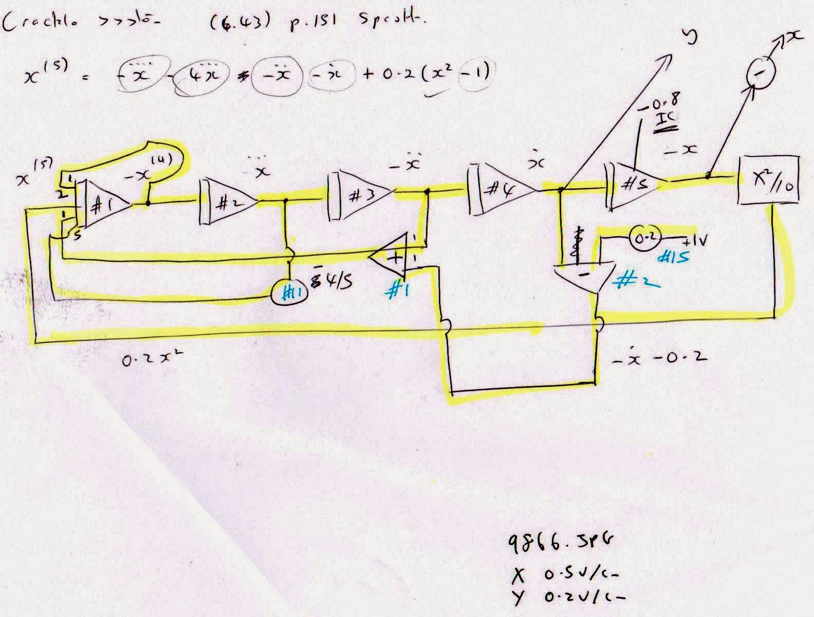
I came across [1] the Rucklidge oscillator, the equations for which are:

In the above, I've included a scaling parameter α (setting α = 1 gives the original equations; for my computer, setting α= 5 gave an appropriate down scaling of the solution (so it fits within +/- 10 V)).

Reference [1] gives results for various values of constants κ and λ - the behavior of the solution depends strongly on these - in particular, it is interesting to plot the solution either side of (something called) the homoclinic bifurcation (Figure 6 of reference [1]).

I plotted the results for three values of λ (blue = -2.5; red = -3.15; green = -6.0). In all cases κ = -1.724, (corresponding to Rucklidge's B point).

The blue curve (λ = -2.5) corresponds to region I of reference [1] - a 'gluing bifurcation'; the red curve (λ = -3.15) and green curve (λ = -6.0) are in region II - a 'homoclinic explosion'. All solutions share the same initial condition (v0 = 0.4). Evidently, the solution does indeed descend into chaos, as λ is made more negative.

Fascinating stuff.

vw-plane (w is vertical), both axes 0.2 V/cm

uw-plane (w is vertical), both axes 0.2 V/cm

Reference

[1] Rucklidge, A.M. (1992) Chaos in models of double convection. Journal of Fluid Mechanics, 237. pp. 209-229.

Ueda

So far I've looked at undriven systems.

The periodically driven Ueda oscillator is described thus [1]:

Here the thing has a sinusoidal driving term on the right hand side. I naïvely thought that this term should be had by integrating 1 volt (actually minus one volt) - to yield t - and then taking the sine of it...but then after some thought I realised that this sinusoidal term can be cooked up more elegantly (and importantly without any limit on t) by solving another differential equation:

 with initial conditions z = 0 and dz/dt = 1. This gives the solution

Scaled equations (by a factor of two).

Patching diagram.

The problem was set up for the parameters used in reference [1], a = 7.5, b = 0.05 and ω = 1. Initial condition was x0 = 2.5.

Below (red plot) is the result (0.2 V/cm horizontal axis (x) and 0.5 V/cm vertical axis (y)). The left hand blue plot is taken from reference [1]:

Reference

[1] Dumitru Deleanu, Description of strange attractors using invariants of phase-plane, Proc. 13th WSEAS Conf. on mathematical methods, computational techniques and intelligent systems, 2011, pp. 113 - 116.

Pierre François Verhulst

I've had a look at the (Verhulst / logistic differential equation):

(with unit growth rate and carrying capacity equal to 10), which has solutions:

Implementation was straightforward.  To get time (as a voltage - to plug into the scope's horizontal axis), I just ran one integrator with unit input (1 volt) - so its output is (negative) t.

To get the set of discrete initial conditions (1 V, 2 V, etc) I connected the new asynchronous reset jack (see earlier post) to the output of an equality test of ⌈x⌉ = x, where x is the ramp voltage, and ⌈x⌉ is the smallest integer not less than x. One of the integrator's ICs was then connected to ⌈x⌉ (the other integrator which gives t has its IC connected to 0 V, so t runs 0 to 10 volts for each different IC).

The computer was run in repetitive (REP) mode. At the start of the REP mode cycle, the initial condition will be set to 0 V. As the ramp voltage x increases, the output of ⌈x⌉ will equal 1 V and when the ramp voltage equals 1 V, the equality  ⌈x⌉ = x will be true and the integrator's initial condition RESET to 1 V; the output of the ⌈x⌉ will now be 2 V and so on. The differential equation is thus solved for each IC in turn. A final touch was to connect the oscilloscope's z-axis to the computer's RST output jack - this goes high (+10 V) when the computer's integrators are being reset (either via asynchronous jack input or at end of REP mode cycle). This rids us of flyback traces on the scope's display. And the result is:

1 V/div horizontal axis; 2 V div vertical axis. Lowest curve is for 1 V initial condition.

Compares with the actual solutions:

A commodius vicus of recirculation...

Perhaps this really is the final bit of circuitry - back to where I started all of this and a revised power supply:

This new one - which uses LM138 and LT1033 regulators - has a short (100 ms) switch-on delay for the negative rail and electrolytics with a higher working voltage.










And an opportunity for a new livery for the control rack's front panel (with its new asynchronous RST jack):

It is a bad plan that admits of no modification...

In its original guise, the computer forces a RESET of the integrators at the start of each REP mode cycle. It occurred to me that it would be useful to be able to reset the integrators in an asynchronous fashion - i.e. to be able to force one or more RESETs during the REP mode cycle.  Why? Because then I can patch the initial condition (IC) jack of the integrator(s) to the 0 - 10 V REP mode ramp output, and force RESETs when (for example) the ⌈x⌉ = x, where x is the ramp voltage, and ⌈x⌉ is the smallest integer not less than x. (The computer has the ceiling (and floor) function available, plus equality tests.)

Hence, at the start of the REP mode cycle, the initial condition will be set to 0 V. As the ramp voltage x increases, the output of ⌈x⌉ will equal 1 V and when the ramp voltage equals 1 V, the equality  ⌈x⌉ = x will be true and the integrator's initial condition RESET to 1 V; the output of the ⌈x⌉ will now be 2 V and so on.

In this way, the integrator's IC jack can be set to 0 V, 1 V, 2 V... and so on, the integrator being RESET each time, computation continuing until the next RESET, and the whole thing repeating once the ramp voltage equals 10 V.

That's the theory anyhow.

To do this I've modified the ramp board circuitry. The easiest approach was to have a little board with a couple of CD4001 NOR gate chips, which is wired to a 14 pin header which replaces the CD4011 (NAND gates) chip on the ramp board (see http://analog-ontology.blogspot.co.uk/2013/07/ramp-board.html):

(Truth table cooked up - converted to minimal forms - the cheapest of these picked (NOR gates) - this is the only bit of the computer's circuitry simulated on a (digital) computer!)

The most annoying thing is the requirement for a new jack on the front panel (and thus new front panel):

In hindsight, it would be better to give each of the integrators its own RST jack - these could then be plugged as required into a common RESET line.

Snap, Crackle and Pop

Crackle

Pop (0.5 V/div) FAST mode

Crackle (X axis 0.5 V/div, Y axis 0.2 V / div) FAST mode

Pop

Snap

Equations taken from Sprott, figures 6.22 (CS2), 6.23, and 6.24 respectively:

With my patchings:

Pop patching for Sprott Figure 6.24.

Snap patching for Sprott Figure 6.22.

Crackle patching for Sprott Figure 6.23.

Complex Systems

It is apparent that certain chaotic systems can be written in a rather compact fashion using complex notation. For example AC6 and AC7 from Sprott (page 157):

where z = a + ib.

Since the imaginary part is just that - imaginary - I cannot deal with it directly on my (real) computer. So after a little algebra we re-cast from the compact to the less than compact pair of equations:

where, in the second equation, the plus sign corresponds to AC6, and the minus sign to AC7. At least now we can imagine that the imaginary part is real (i.e. b).

Interestingly, this is a real mess to patch together (in the real world) - perhaps this says something about the universe...

Incidentally, this is the first time I've used the computer's power functions (to get the cubes) - via AD538s.










Initial conditions are a = 0.5, b = 0.5; their first derivatives are zero. And my state space plots:

AC6

AC7

Both plots: b is vertical and a horizontal (equal scales throughout: 0.2 V/cm.)


These compare nicely with Sprott's Fig 6.28.